Hidden watermark
A practical guide to finding and nuking hidden watermarks in screenshots.
OS tool installation
| Tool | Why | install | Command |
|---|---|---|---|
| exiftool | strips metadata | sudo apt install -y libimage-exiftool-perl | exiftool -all= -overwrite_original demo.png |
| ImageMagick | re-encodes, resizes, blurs, inverts, compares | sudo apt install -y imagemagick | See Commands Cheat Sheet |
| zsteg | PNG/GIF/BMP LSB checks (not JPG, not WebP, etc.) | sudo apt install -y ruby-full && sudo gem install zsteg | zsteg -a demo.png |
| binwalk (Optional) | Peeks inside any binary/firmware & extracts hidden blobs. Overkill for screenshots, but handy for occasional firmware/APK spelunking. | sudo apt install binwalk | binwalk -e demo.png |
Detect Douban screenshot
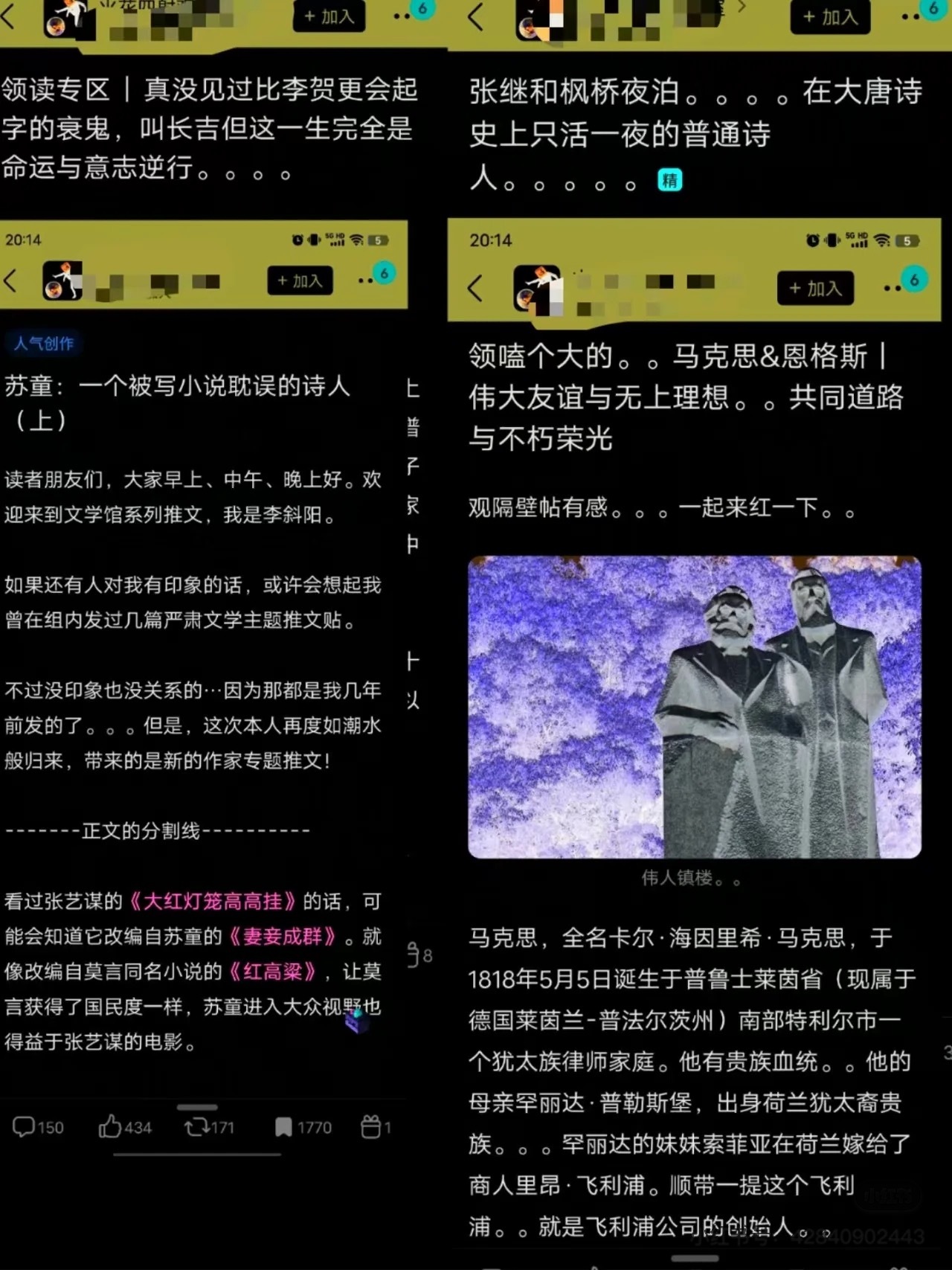
Back in 2022
Screenshots were embedded with plaintext watermarks, easily visible as soon as you applied a simple filter:
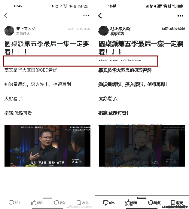
Zoom in:
fully readable metadata looks like:
uid: 34652544 tid: 255645623 time: 2022-12-19T16:48:29+08:00
(my eyes hurt)
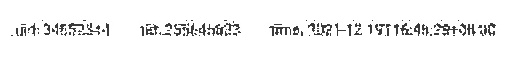
This is exactly what was discussed in this 2022 Zhihu post:
- Format:
uid: [UID] tid: [TID] time: [TIMESTAMP]`
It’s just three fields, with spaces (or tabs) between them, and no JSON/curly braces, just raw text.
Today
Now, the watermarking has become encrypted and more stealthy. So what we’re doing here is detection = not extraction.
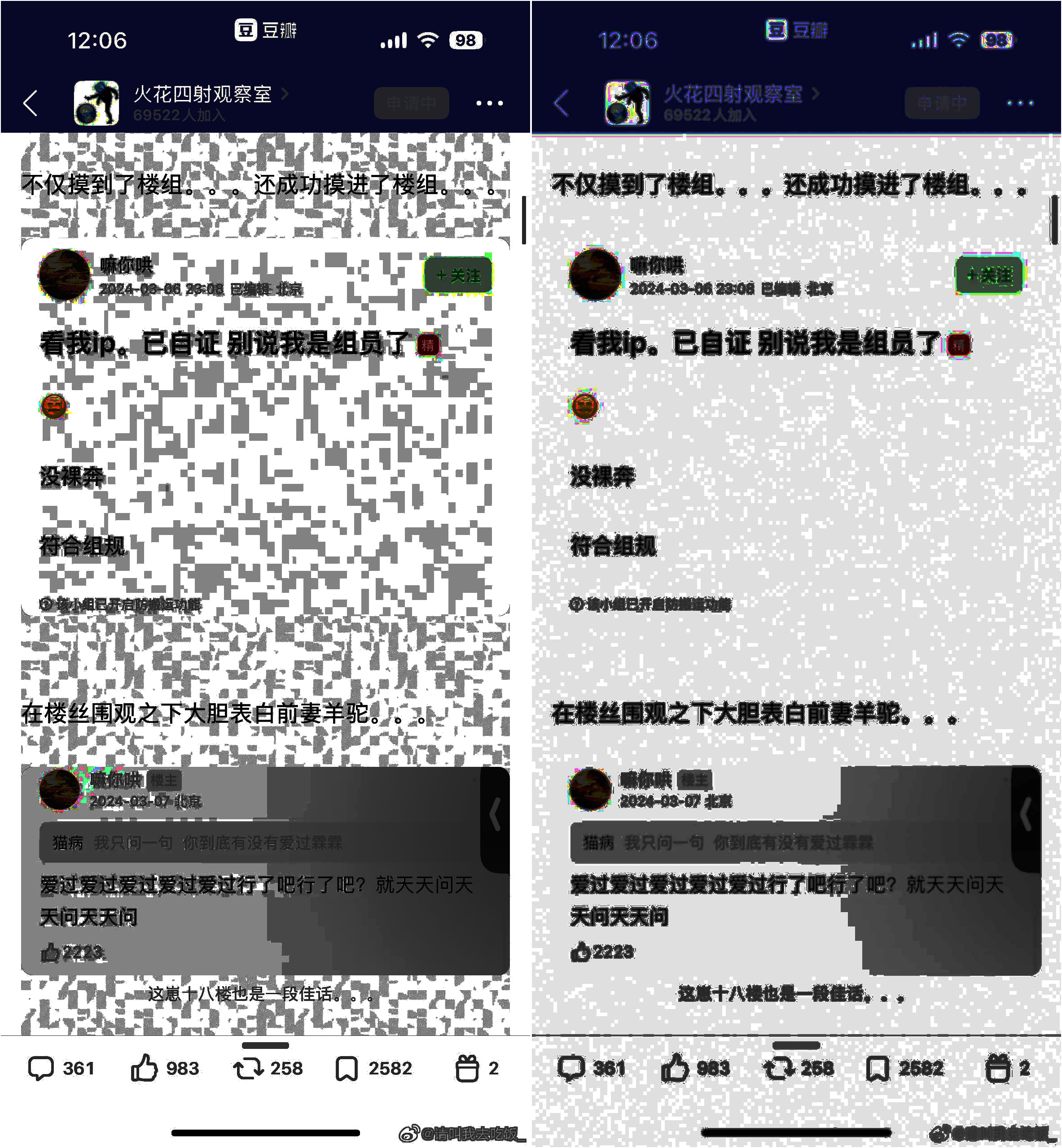
Here’s the demo sample we’re working with:
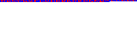
To reveal:
1
convert demo.png -channel RGB -negate demo_inverted.png
This image reveals a subtle pattern in the background,
but it’s only visible if you zoom in:
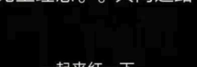
1
convert demo.jpg -equalize demo_eq.jpg
That should give you the clearest view of the snow pattern:
How do they track
In certain groups, Douban would explicitly stated that when you take a screenshot of a group post, it will automatically embed an encrypted user ID, post ID, and timestamp directly into the image.
Likely pipeline:
- Server decides the watermark mask from your UID / post-ID / timestamp. (Could be a 1-bit pseudo-random matrix seeded with a hash.)
App (iOS/Android or web Canvas) draws:
┌─────────── Screen Layer Stack ───────────┐ │ UID-snow mask (alpha ~3-5 %) │ ← NEW │ Article text & images │ │ Background │ └───────────────────────────────────────────┘- Implementation: tiny fragment shader, or
Canvas.drawBitmap(mask, PorterDuff.ADD), or CSSmix-blend-mode.
- Implementation: tiny fragment shader, or
- When you hit screenshot, the OS composites all layers → PNG. Your file already has the mask, so any equalize shows snow.
How They Encode the UID
A common recipe they might use (one of several):
Generate a pseudorandom bit-plane:
1
2
 rng = np.random.default_rng(hash(uid+post_id+timestamp) & 0xFFFFFFFF)
 mask_bits = rng.integers(0, 2, size=(screen_h, screen_w), dtype=np.uint8)
Convert to ±Δ luminance and apply to each RGB channel:
1
2
3
 delta     = 2          # 1-3 is enough: invisible to eye
 overlay   = (mask_bits*2 - 1) * delta   # 0→-Δ , 1→+Δ
 rgb[:]    = np.clip(rgb + overlay[...,None], 0, 255)
Repeat or tile if the post scrolls longer than one screen.
It’s NOT LSB stego. The watermark rendered by CSS(If it’s a web app) is visible, even if faint. It is a front-end overlay, not an embedded digital stenography like LSB, DCT, or EXIF fingerprint. But it can lead to LSB or fingerprint-style traps later. Some apps take it further:
- Render a CSS-based watermark
- Then apply client-side canvas tricks to rasterize it subtly
- OR use a CDN to deliver a pre-fingerprinted image per user
- THEN use LSB-like techniques to alter the final rendered raster
So what looks like “just CSS” can actually become user-specific invisible traces, depending on how the browser rasterizes it.
| Technique | Source | Visible | Affects Screenshot | Can Leak User ID? |
|---|---|---|---|---|
| CSS watermark | front-end style | Semi-visible | Yes | Yes if tied to user ID |
| Background-image with Base64 | front-end | Barely visible | Yes | Yes |
| Canvas drawing (JS) | front-end | Maybe | Yes | Yes |
| Stego images (LSB, DCT) | CDN-delivered | Invisible | Yes | Yes |
| Font fingerprinting (anti-screenshot shapes) | CSS/JS | Hidden in rendering | Yes | Maybe indirectly |
If we don’t peek into the app’s backend APIs, it really feels like a black box.
Since we still don’t know exactly what technique was used for the hidden watermark, we shouldn’t assume that methods like:
1
convert demo.png -channel R -separate +channel -threshold 50% demo_R.png
will actually remove it (in output image). This only works for basic LSB-based watermarks. And it won’t keep color either, only black and white.
-threshold
1
convert image.png -threshold 50% output.png
Takes every pixel → checks its brightness →
If brightness ≥ 128 → becomes white (255)
If < 128 → becomes black (0)
This is NOT just affecting LSB, but kills all bits above or below the threshold. It won’t keep colors. Even if:
1
-channel R -threshold 50%
It still produces a grayscale image, not red anymore. It’s always monochrome after thresholding.
So equalize after threshold won’t help, either. Since after threshold, we’ve already reduced the image to just black and white. There’s no contrast to stretch anymore.
LSB
image files, especially PNGs, have 8 bits per color channel per pixel. So for every pixel’s red value:
Bit position:   8  7  6  5  4  3  2  1
                ↓  ↓  ↓  ↓  ↓  ↓  ↓  ↓
Binary value:   1  0  0  0  1  1  0  1  (which is 141 in decimal)
Bit weight:   128 64 32 16  8  4  2  1
                ↑                    ↑
  MSB (Most Significant Bit)  LSB (Least Significant Bit)
That last bit barely changes color (±1 out of 255), so your eyes can’t tell. But computers can. And that’s exactly where companies hide payloads like tracking info, encrypted IDs, even watermarks.
LSB Steganography Hands on
Let’s try to hide a secret message (like your UID, post ID, time) inside a screenshot by changing the least significant bit (LSB) of each pixel in the top part of the image. This method is called LSB steganography or LSB Embedding = it tweaks the tiniest part of the color so the human eye can’t see the difference, but a computer can always extract it if it knows where to look.
LSB Embedding
Make the secret message
We want to hide this information:
1
2
3
4
5
 payload = {
   "uid": "123456789",
   "tid": "260239564",
   "ts": "2025-07-01T12:32:57"
 }
which includes user ID, thread/post ID, and a timestamp.
Turn the message into binary
Computers work with 1s and 0s, not text, so we need to encode the message. First, turn it into a single string using JSON:
1
2
 payload_str = json.dumps(payload)
 # '{"uid":"123456789","tid":"260239564","ts":"2025-07-01T12:32:57"}'
Then, turn every character into its 8-bit binary form:
1
2
3
 bits = ''.join(f'{ord(c):08b}' for c in payload_str)
 # If the string was 'A', ord('A')=65, bin(65)=01000001
 # So 'A' → 01000001
Finally, add
'00000000'at the end as a null terminator = so our decoder knows where to stop.Try this
json2bit.pyfrom my repo. It shows exactly how a JSON payload turns into a clean LSB-ready bitstream:1 2 3 4 5 6 7 8 9 10 11 12 13 14 15 16
Original JSON string: '{"abc": 1}' Character breakdown: '{' → ord: 123 → bin: 01111011 '"' → ord: 34 → bin: 00100010 'a' → ord: 97 → bin: 01100001 'b' → ord: 98 → bin: 01100010 'c' → ord: 99 → bin: 01100011 '"' → ord: 34 → bin: 00100010 ':' → ord: 58 → bin: 00111010 ' ' → ord: 32 → bin: 00100000 '1' → ord: 49 → bin: 00110001 '}' → ord: 125 → bin: 01111101 Full binary bitstring (with end padding): 0111101100100010011000010110001001100011001000100011101000100000001100010111110100000000
Embed the bits in the image’s pixels
The image is like a big table of pixels. Each pixel has a red, green, blue value (0~255). We take the red channel of the top 32 rows, flatten it into a long 1D list, and for each bit of our message:
- Change the last bit (the LSB) of that pixel to be 0 or 1 depending on our message.
Example:
If pixel red value =
10110010(178 in decimal), and next secret bit =1, set pixel red =10110011(179 in decimal)If secret bit =
0, set last bit to 0:10110011→10110010(back to 178)
1
 flat[i] = (flat[i] & 0b11111110) | int(bit)
flat[i] & 0b11111110zeroes out the last bit.| int(bit)sets it to the secret bit.
We do this for each bit of the message and each corresponding pixel.
Btw, a quick cheat sheet for bitwise comparison
 | Operation | Binary Result | Decimal |
 |-----------|----------------|---------|
 | A         | 10101010       | 170     |
 | B         | 11001100       | 204     |
 | A & B     | 10001000       | 136     |
 | A | B     | 11101110       | 238     |
 | A ^ B     | 01100110       | 102     |
 | ~A        | 01010101       | 85      |
 | ~B        | 00110011       | 51      |
 | NAND      | 01110111       | 119     |
 | NOR       | 00010001       | 17      |
Save the watermarked image
We put the edited red-channel pixels back, and save the image as a new PNG file.
See the complete LSB embed code for R channel here(lsb_embed_R.py), which uses a tiny 4x4 image as an example.
Also see:
Write/Decode different LSB bits to/from each channel:
Write/Decode the same bits to/from all channels:
People can’t see the difference with eyes = the image looks exactly the same. But if you extract the red-channel LSBs in the right order, you get your hidden message back. LSB embed is very old school (kinda like talking about 90s zines, hehe), one of the earliest, simplest forms of digital steganography.
Decode LSB Embedding
See lsb_decode_R.py
Or just use:
1
2
# sudo apt install -y ruby-full && sudo gem install zsteg
zsteg -E b1,r,lsb hidden_demo.png | strings
It’ll directly output:
{"uid": "123456789", "tid": "260239564", "ts": "2025-07-01T12:32:57"}
To decode, we read back the LSB of each pixel in the same order, so we get the message bits back out.
Key line:
1
bits = ''.join(str(px & 1) for px in flat)
It extracts the secret message from the image by grabbing the last bit (LSB) from every red pixel = in the same order we hid them.
Go through each pixel value in the red channel, in order. Then px & 1 uses bitwise AND to get just the last bit of each pixel’s value.
- If px ends with 0 (
...0),px & 1= 0 - If px ends with 1 (
...1),px & 1= 1
So we know whether the last bit of each pixel a 0 or a 1.
Say we got '011110110111110100000000' after this. That’s the binary for '{}' plus the null terminator (00000000).
Then in decoding loop,
1
2
3
4
5
6
7
8
9
10
chars = []
for i in range(0, len(bits), 8):
    byte = bits[i:i+8]
    if len(byte) < 8:
        break
    val = int(''.join(byte), 2)
    if val == 0:
        break
    chars.append(chr(val))
msg = ''.join(chars)
we loop through the bit string 8 bits at a time (1 ASCII character = 8 bits).
byte = bits[i:i+8]grabs the group of 8 bits (e.g.,'01111011').val = int(''.join(byte), 2)converts the 8-bit string into an integer. For'01111011', this gives 123 (which is ASCII for'{').if val == 0: breakstops until we hit the null terminator (00000000→ 0), which means no more message left.chars.append(chr(val))turns the number into a character, add to the list.- 123 →
'{' - 125 →
'}'
- 123 →
- Then we finally get the original hidden message with
msg = ''.join(chars). (in this example,'{}')
Visualize LSB Embedding
Now we can make the area where the watermark lives visibly marked (e.g., filled with red or any color) so a human can see exactly where the secret is hidden.
Make “1” bits red, “0” bits blue:
1
2
3
4
5
6
7
8
9
10
11
12
13
14
 arr = np.array(Image.open("hidden_demo.png"))
 flat = arr[:32,:,0].flatten()
 payload_bits = ''.join(f"{ord(c):08b}" for c in '{"uid": "123456789", "tid": "260239564", "ts": "2025-07-01T12:32:57"}') + '00000000'

 for i, bit in enumerate(payload_bits):
     if i >= flat.size: break
     y, x = divmod(i, arr.shape[1])
     if bit == '1':
         arr[y, x] = [255,0,0]  # red for 1
     else:
         arr[y, x] = [0,0,255]  # blue for 0

 img3 = Image.fromarray(arr)
 img3.save("hidden_demo_colored.png")
y, x = divmod(i, arr.shape[1])actually does:1 2
row = i // arr.shape[1] col = i % arr.shape[1]
i: the index of the bit in payload stringarr.shape[1]: the width of the image (number of columns)- Going row-by-row, left to right, top to bottom
Say an image is 1280px wide, and you’re on the i = 1300th bit:
1
 divmod(1300, 1280) ➜ (1, 20)
So
y = 1,x = 20, the pixel is at row 1, column 20.The output “hidden_demo_colored.png” would be like this:
Note the top 32 px are colored.
equalize & stretch help, fast and dirty!
1
 convert hidden_demo.png -auto-level -contrast-stretch 1%x1% hidden_demo_stretch.png

1
 convert hidden_demo.png -equalize hidden_demo_eq.png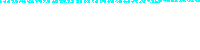
Since we only embed data in R channel, if we separately equalize every channel, ofc we would only see the noise in R channel:
1
2
3
 convert hidden_demo.png -channel R -separate -equalize r_eq.png
 convert hidden_demo.png -channel G -separate -equalize g_eq.png
 convert hidden_demo.png -channel B -separate -equalize b_eq.png
Then use
montageto compare R, G, B channel in order:1
montage r_eq.png g_eq.png b_eq.png -tile 3x1 -geometry +2+2 -background "#1e1e1e" rgb_eq_cmp.png

The difference between these two “equalize” ways
-auto-level -contrast-stretch 1%x1%1
convert hidden_demo.png -auto-level -contrast-stretch 1%x1% hidden_demo_stretch.png
-auto-level:- Stretches the darkest pixel to black (0), lightest to white (255).
- Everything else is linearly scaled.
No fancy histogram tricks = just pushes the endpoints out.
-contrast-stretch 1%x1%:- Cuts off the darkest 1% and lightest 1% of pixels (ignores outliers), then scales the rest.
- Boosts contrast but mostly preserves linear relationship.
- Good for fixing under/overexposed photos.
Stretches overall contrast, makes normal photo details pop, but doesn’t aggressively expand small changes (like LSB-only edits) unless those are significant compared to the rest of the image.
-equalize1
convert hidden_demo.png -equalize hidden_demo_eq.png-equalize:- Stretches and evens out the contrast of the image, so darks become lighter, lights become darker, and “midtones” spread out.
- Makes the histogram flat (tries to distribute pixel values equally across all levels).
- Aggressively stretches small intensity differences, especially in regions with little contrast.
- So even the tiniest clusters of pixel values (like those caused by a blind watermark) are exploded into visible patterns/noise.
Even tiny variations, like those from watermark LSB tweaks, become very visible, way more than with auto-level/contrast-stretch.
-equalizeworks better for watermark bands- The watermark only slightly changes pixel values (often only 1 gray level out of 255).
-auto-leveland-contrast-stretchmight ignore such tiny differences if the rest of the image has normal contrast, because they only care about endpoints and global range.-equalize, though, stretches every little difference into a visible gap = even if it was just a single-bit tweak in a big field of similar pixels.
So if watermark band is super subtle, we’ll see almost nothing with -auto-level -contrast-stretch, but -equalize helps the hidden “barcode” band jumps out.
Limitation
These 2 “equalize” methods only reveal certain types:
- LSB-based steganography.
- Watermarks that are just “low contrast” bars/bands, or slight repeated pixel tweaks in one channel.
What WON’T be revealed:
- Spread-spectrum, frequency-based stego: Where data is hidden as patterns across the entire image, not just in low bits or a specific band.
- DCT/transform-domain steganography: (e.g., JPEG stego, where info is encoded in frequency coefficients, not pixel color directly).
- Color channel shuffling: Some stego hides info only in green/blue or even in alpha, or across channels in a key-based way.
- Encrypted or heavily dithered data: If the encoded bits are completely randomized and mixed in, you’ll just see uniform static, not a barcode.
- Invisible watermarking: Some pro methods change the image statistically so that only their own proprietary tool can read the watermark.
Verdict
Before they just drew those watermark characters (uid/tid/time) as super-low-opacity white or gray text on top of the screenshot. So if you raised the curves or levels, invert, etc, you could suddenly see faint letters pop up. You could read the UID/TID/TIME as actual text. Some phones (like Redmi) with special dark mode or boosting contrast would also reveal these.
Now, instead, We won’t see the actual text with any visual filter, curve, dark mode, Photoshop, etc, unless extract the bits in code and then decode them back to characters. What we’ll see with extreme filters is weird blocky snow patterns, but never the actual number or text. This “noise” just shows the distribution of bits (not the data itself), but never readable.
Douban’s snow/lego watermark is truly a pixel-level, visible overlay - not an invisible LSB/DCT/metadata trick. It’s rendered on top of the entire post. The watermark is “baked in” before you even get the image file.
Taking a screenshot of a screenshot app window does NOT break the pattern, because the pixel arrangement is copied exactly Rephotographing (using a phone/camera to take a physical picture of your monitor) DOES break it! Because the camera lens, sensor noise, color calibration, etc, all introduce analog “noise.” The pixel-perfect alignment is lost. Equalization can’t revive the old pattern, since it’s not the exact same pixels anymore.
After LSB
Now if we try to read the LSBs to extract something from Douban screenshot, you’ll get a lotta ÿ, which is Unicode for 0b11111111 (decimal 255). Or you get many “extended ASCII” (ü, û, ½, ß, etc). So I guess it’s likely:
- Random/noise: if their watermark is encrypted or obfuscated, we’ll get junk/garbage, e.g., all 1s (
ÿ), all 0s (\x00), or mixed symbols. - Obfuscation: encrypted/hashed/randomized.
- Not plain text: They may encode info as numbers, then encrypt it, then embed.
- Spread out: Could be interleaved across channels, or bits split over whole image, or even with error correction codes.
So watermark IS present (those Lego-snow patterns prove it), and all three channels hold data, but it’s NOT stored as ASCII/plain text anymore. They could be interleaved/compressed/encrypted, etc, could be using more than just LSB.
Anyway, let’s try LSB extraction.
Douban only embed the watermark when there’s a new screenshot session (like restart the APP), not on every single screenshot. If re-screenshot the exact same group/post at the same session, their server might re-use the previous payload. In same post(same uid, same tid), different time, LSB changes appear farther down the gibberish stream. It’s likely they encode static stuff (UID, TID) at a certain offset, and dynamic stuff (timestamp) at a later offset (or vice versa).
Shannon entropy
Shannon Entropy is a way to measure uncertainty or surprise in a stream of data.
Say you’re reading a sentence, and every character is super predictable, like:
1
AAAAAAAAAAAAAAA
You already know the next letter is “A”, which is low entropy.
- High entropy = lots of randomness (hard to guess what’s next)
- Low entropy = very repetitive (easy to guess)
So in hidden watermark or steganography, if entropy is too low, it’s probably repetitive filler. If it’s medium, it could be normal readable data. If it’s very high, it’s likely encrypted or compressed.
- Natural language (like English text) tends to have moderate entropy.
- Code/JSON/logs might be slightly higher entropy than plain English, but still lower than encrypted or compressed data.
- Encrypted or compressed blobs aim to be as close to totally random as possible, maximum entropy.
We can calculate how random the LSB is, using Shannon entropy. Then check if the decoded message might contain something readable like "uid" to help us guess if it’s plaintext vs gibberish.
1
    return -sum((c/len(data))*math.log2(c/len(data)) for c in freq.values())
This line is a literal translation of the core entropy formula:
\[H = - \sum_{i} p_i \log_2 p_i\]Where $p_i$ is the probability of each byte value, and it says how common something is.
- $c$ is the count of a symbol (like how many times ‘A’ appears)
- $\frac{c}{\text{len(data)}}$ is the probability $p_i$ of that symbol
math.log2(): log base 2 of that probability, which gives a weight to the surprise
Looping through each unique byte in data, and calculating how much surprise it brings.
So $p_i \log_2 p_i$ makes common symbols contribute less info; rare ones contribute more. And the final negative sum gives the total entropy.
Say the message is:
1
b'AAAAAA'
Frequencies:
- A = 6
- Total = 6
So:
- $p = 6/6 = 1.0$
- $H = -1.0 \cdot \log_2(1.0) = 0$ ← no surprise
Another message is:
1
b'ABCDEF'
All letters different:
- $p = 1/6$
Each symbol contributes:
\[-\frac{1}{6} \cdot \log_2\left(\frac{1}{6}\right) \approx 0.43\]- Total entropy ≈ 2.58
Here’s a quick cheat sheet for entropy reference:
Low entropy (≈0-2):
- Often: All-zeros, repeated chars (e.g.,
ÿÿÿÿ), or simple repetitive watermark. - Or: Short readable messages (ASCII only, English text).
- Often: All-zeros, repeated chars (e.g.,
High entropy (≈4-8):
- Often: Random-looking data, encrypted or compressed payload.
- Or: Large readable payload with wide character distribution (mixed case, numbers, symbols).
“Normal” readable English:
- Text: Typically 4.0-5.0
- Pure random: Up to 8.0 (full 8-bit spread)
Like the JSON (e.g. '{"uid": "123456789"...}') mixes curly braces, quotes, numbers, colons, a pretty rich charset, would bump up entropy. Short readable messages can seem high-entropy if they contain diverse chars. A file of only “a” or only “ÿ” would be nearly zero entropy.
Check this script here (entro_checker.py).
If most files have entropy between 0.01-1.2 and decoded message length in the thousands, but never anything readable, never uid, then almost certainly these images are either not using LSB-watermarking at all, or their method is heavily obfuscated (random or constant pattern, or not in the LSB at all). Or your screenshots are compressed JPGs, which destroys most LSB stego.
If everything is always low-entropy, low-printable, or blank - safe from “plain” uid leaks via screenshot, at least in LSB…
bit-planes
Every grayscale (or color channel) image pixel is stored as an 8-bit number. Like:
1
Pixel value: 156 → binary: 10011100
Each of those 8 bits, from the most significant bit (MSB) to the least significant bit (LSB), forms a bit-plane.
- Bit-plane 7 (MSB) = first bit (highest weight)
- Bit-plane 0 (LSB) = last bit (lowest weight)
For a 512×512 image, we can split it into 8 “images”, each one showing what all the pixels look like at one specific bit position. That’s the bit-plane view.
Because 1 byte = 8 bits. Most images are stored using 8-bit integers per channel:
- Grayscale: 1 channel = 8 bit-planes
- RGB: 3 channels = 8×3 = 24 bit-planes
Each bit controls 2ⁿ value range:
| Bit Position | Weight | Effect |
|---|---|---|
| 7 (MSB) | 128 | Controls brightness chunk |
| 6 | 64 | Large visible impact |
| 5 | 32 | Medium impact |
| … | … | … |
| 1 | 2 | Tiny visual detail |
| 0 (LSB) | 1 | Great for hiding secrets with little impact visually |
visualize all bit-planes (R/G/B)
- visible detail comes from (MSB=leftmost)
- noise or stego data might be lurking (LSB=rightmost)
Here are some ways to visualize:
Let’s try bit_planes.py:
The last two bit planes of all three channels show an obvious snow-like pattern.
Use steghide to hide info in jpeg
steghide uses symmetric encryption internally (default: AES). Works with JPG, BMP, WAV, AU, but NOT PNG. steghide scrambles bits and embeds based on statistical matching, not straight LSB. LSB analysis won’t help here. Only with wordlists or bruteforce tools like steghide-brute-force (not built-in).
Its passphrase is used to:
- Derive the key
- Decrypt the embedded payload (file, text, zip, whatever)
Install steghide:
1
sudo apt install -y steghide
Embed (aka hide) secret.txt into demo.jpg:
1
2
steghide embed -cf demo.jpg -ef secret.txt
# It'll prompt you to create a passphrase
-cf demo.jpg: Cover file - the image you’re hiding inside-ef secret.txt: Embed file - the thing you’re hiding- (prompted)
Enter passphrase:Used to encrypt and lock the payload
Steghide encrypts secret.txt. It embeds the encrypted data into statistically safe places inside demo.jpg The output overwrites demo.jpg unless you add -sf output.jpg. So now, demo.jpg looks normal, but it secretly contains your secret.txt, locked with a passphrase.
Then try:
1
steghide info demo.jpg
Check if the image has embedded data (without extracting it yet)
It tells the format, capacity, and whether there’s hidden data. If yes, it’ll prompt:
  Try to get information about embedded data ? (y/n) y
  Enter passphrase:
With the right passphrase, it’ll tell you the name/type of embedded file (optional metadata), like:
  embedded file "secret.txt":
    size: 11.0 Byte
    encrypted: rijndael-128, cbc
    compressed: yes
Then try:
1
steghide extract -sf demo.jpg
to extract (aka recover) the hidden file from demo.jpg.
-sf demo.jpg: Stego file - the image that contains hidden content
You’ll be prompted:
Enter passphrase:
If correct, the original secret.txt is recovered in the current folder.
After steghide extract, the demo.jpg is NOT the same as before. Even after extraction, demo.jpg still contains the hidden data. Because steghide extract just copies the hidden file out, but it does not touch or “sanitize” the image. demo.jpg still contains the full encrypted blob inside.
Try to test this with:
1
sha256sum demo_raw.jpg demo.jpg
It’ll output totally different hashed:
eaf9cdca6fd91as4b4af74a5c5e64c55978b8e891223d7e898007c1a14fddd60  demo_raw.jpg
945b6c56e025acy7f2a73df3433733f5287a0ae424cdaf179cdfb131c5d1d699  demo.jpg
DCT (Discrete Cosine Transform)
DCT is like turning an image into its musical notes.
Say you got a square of pixels, like a tiny 8×8 patch from your screenshot. Now instead of looking at the brightness of each pixel one-by-one, DCT goes: “how much of this square looks like a wave going left to right? What about top to bottom? Or a checkerboard pattern?” It breaks that image patch into a combo of frequency waves, like turning it into a chord instead of individual notes.
LSB hides data pixel by pixel, it’s weak when we JPEG or resize it. DCT hides data in frequency land. Compression can’t easily ruin it.
DCT is the heart of JPEG. Every time you save a JPEG, DCT is what your image goes through before it gets smushed into those tiny files. That’s why watermarking inside DCT blocks is:
- invisible to the eye
- harder to kill with basic edits
- easier to embed a bit of ID or fingerprint
How DCT works with JPEG
JPEG divides your image into 8×8 blocks
Say you have a grayscale image (just for simplicity). Every 8×8 block of pixels is like a little tile. Each tile contains 64 values (brightness: 0-255). JPEG processes each tile independently. The whole image is like a bathroom wall covered in mini-tile stickers, and each tile is analyzed on its own.
DCT transforms each tile into frequencies
This is where DCT comes in. It converts those 64 numbers (brightnesses) into 64 new numbers. Now those numbers represent frequencies.
- Top-left corner of DCT block = DC coefficient = average brightness
The other 63 values = AC coefficients = frequencies:
- Horizontal waves
- Vertical waves
- Diagonal waves
- The higher you go in the matrix, the higher the wave “wiggle” rate.
 # JPEG DCT Block Layout (8x8)
 # Each element represents a frequency component

 [
   DC,   H1,   H2,   H3,   H4,   H5,   H6,   H7,  ← increasing horizontal freq →
   V1,   D1,   D2,   D3,   D4,   D5,   D6,   D7,
   V2,   D8,   D9,   D10,  D11,  D12,  D13,  D14,
   V3,   D15,  D16,  D17,  D18,  D19,  D20,  D21,
   V4,   D22,  D23,  D24,  D25,  D26,  D27,  D28,
   V5,   D29,  D30,  D31,  D32,  D33,  D34,  D35,
   V6,   D36,  D37,  D38,  D39,  D40,  D41,  D42,
   V7,   D43,  D44,  D45,  D46,  D47,  D48,  HF   ← increasing vertical freq ↓
 ]

 # frequency map

 V +----------------------------------+
 e | DC  ...          Hi-H & Low-V    |
 r | ...              ...             |
 t | ...              ...             |
 . | Low-H & Hi-V     Hi-H & Hi-V     |
 ↓ +----------------------------------+
         Horizontal Frequency →
Position ≠ value. It’s the position in the DCT matrix that tells us if it’s high-frequency in the block.
- DC = Direct Current, low frequency (average brightness)
- H1-H7 = horizontal frequencies (edges left↔right)
- V1-V7 = vertical frequencies (edges top↕bottom)
- D1-D48 = diagonal/complex frequency combos
- HF = highest frequency, wildest, finest details (most “noisy”, sharp edges)
Low-frequency only:
- Smooth gradients
- Blurry, soft, dreamy
- You’d see just outlines, gentle colors
- JPEG compression loves this
High-frequency only:
- Lots of tiny details, sharp edges, text
- Noisy, flickery, harsh
- Very “pixel crunchy”
- JPEG hates this, it nukes the precision here to save space
High-quality JPEGs: keep more of the DCT coefficients, preserve sharpness
Low-quality JPEGs: yeet the high-freq stuff, making the image smaller and softerJPEG quantizes (rounds) these numbers
JPEG knows human eyes suck at seeing high-frequency detail. So it takes the DCT matrix and aggressively reduces precision on higher-frequency areas.
e.g.:
2might become0-1.8might become0DCvalue might be kept more accurately (like103 → 100)
That’s why JPEG compresses better when the image is smooth, those higher-frequency values just die out. JPEG reduces precision on higher-frequency areas. Not turning high-frequency into low-frequency directly, but truncating or rounding off the small details.
Say you have this row of brightness values:
1
 [100, 100, 100, 100, 100, 100, 100, 100] ← flat gray
Its DCT will give:
1
 [800, 0, 0, 0, 0, 0, 0, 0]
Only DC (average brightness) is nonzero.
Another one:
1
 [100, 120, 140, 160, 140, 120, 100, 80]
Is like a wave. Its DCT gives:
1
 [960, -220, 0, 50, 0, 0, -10, 0]
Now we get non-zero AC values, meaning there’s variation (frequency).
- High-frequency = rapid pixel value changes
- Low-frequency = gradual changes
If you hide your watermark in LSB of raw pixel values, it gets wrecked when the JPEG is saved. Because JPEG doesn’t preserve pixel values directly. But if you hide your watermark in DCT coefficients like:
1
embed into bit 1 or bit 0 of a middle-frequency DCT value
then this watermark can survive JPEG compression, even at decent quality settings.
Some kalkulation - blocks & size
In Grayscale (1 channel)
Say the image is:
1
2
Width: 512 px
Height: 256 px
Calc how many 8×8 blocks:
Each 8×8 block covers:
- 8 pixels wide × 8 pixels tall = 64 pixels total
So:
1
2
3
blocks_across = 512 / 8 = 64
blocks_down   = 256 / 8 = 32
total_blocks = 64 × 32 = 2048 blocks
Note:
- The image does not need to be exactly divisible by 8, JPEG will pad it if needed with extra pixels (like zeros).
- But for math, it helps to assume it’s divisible.
In RGB (3 channels)
Each channel (R, G, B) is handled independently for compression.
So for a 512×256 image, we still have 2048 blocks per channel, like in grayscale, but ×3 channels, so:
2048 blocks in R
2048 blocks in G
2048 blocks in B
→ Total of 6144 DCT blocks
BUT JPEG doesn’t always compress RGB directly, it usually converts RGB to YCbCr, then compresses like:
| Channel | Blocks |
|---|---|
| Y | Full res (e.g. 512×256) → lots of blocks |
| Cb | Often downsampled (e.g. 1/2 width & height) |
| Cr | Same as Cb |
Y gets more blocks, and Cb/Cr fewer, since human eyes are more sensitive to brightness than color.
To calculate image size from pixels to MB:
- Pixel count =
width * height - For RAW RGB, each pixel = 3 bytes (R, G, B)
- Divide total bytes to MB:
bytes / 1024 / 1024
e.g.:
Image: 4032 x 3024
1
2
3
4
w, h = 4032, 3024
bytes_total = w * h * 3
megabytes = bytes_total / 1024 / 1024
print(megabytes)  # ~34.9 MB uncompressed
BUT JPEG compresses, so actual size could be 1-5MB, depending on quality.
Quantization Matrix
JPEG uses a quantization matrix = a table that tells how much to divide each frequency coefficient. Higher frequencies get divided harder (i.e., precision gets lost). When high-frequency stuff gets wiped, it’s the first thing to go.
Say a quantization matrix like this:
[1, 2, 4, 8, 16, 32, 64, 128]
Then:
| Original | ÷ Q-table | Rounded | kept (+) / lost (-) |
|---|---|---|---|
| 124 | ÷1 | 124 | + |
| -4 | ÷2 | -2 | + |
| 3 | ÷4 | 1 | + |
| -2 | ÷8 | 0 | - |
| 1 | ÷16 | 0 | - |
| 0 | ÷32 | 0 | - |
| 0 | ÷64 | 0 | - |
| -1 | ÷128 | 0 | - |
Then JPEG rounds these and saves only non-zero.
This is how we get:
1
[124, -2, 1, 0, 0, 0, 0, 0]
On decode, it multiplies the quantization table again and gets back an approximate version of the original matrix.
Quantization matrix is determined by the JPEG encoder software (like Pillow, libjpeg, camera firmware), based on a quality factor (like 90%, 75%, etc). The standard JPEG quantization matrix (for luminance) at quality 50 might look like:
[16 11 10 16 24 40 51 61
 12 12 14 19 26 58 60 55
 14 13 16 24 40 57 69 56
 14 17 22 29 51 87 80 62
 18 22 37 56 68 109 103 77
 24 35 55 64 81 104 113 92
 49 64 78 87 103 121 120 101
 72 92 95 98 112 100 103 99]
Higher values in bottom-right = harder quantization = more loss. The encoder scales this up/down based on the quality setting.
Get your JPEG’s quantization matrix
1
2
3
4
from PIL import Image
im = Image.open("your_image.jpg")
qtables = im.quantization
print(qtables)  # Returns dictionary of quant tables
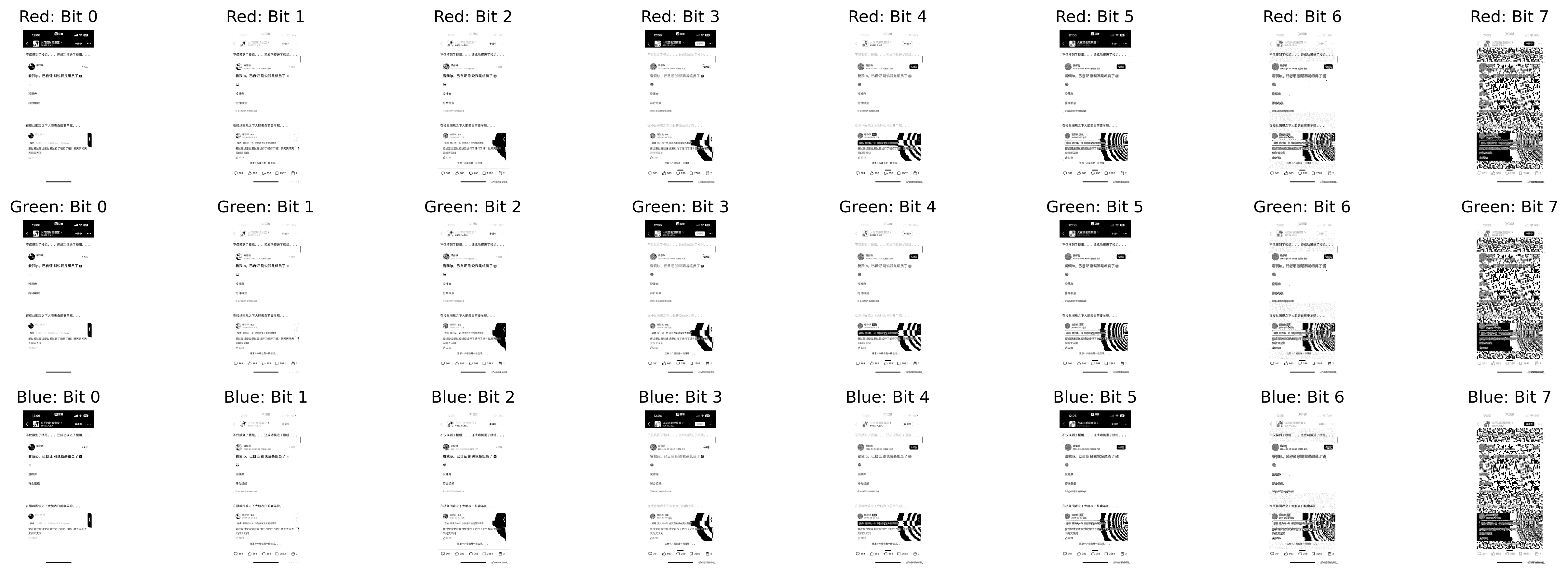
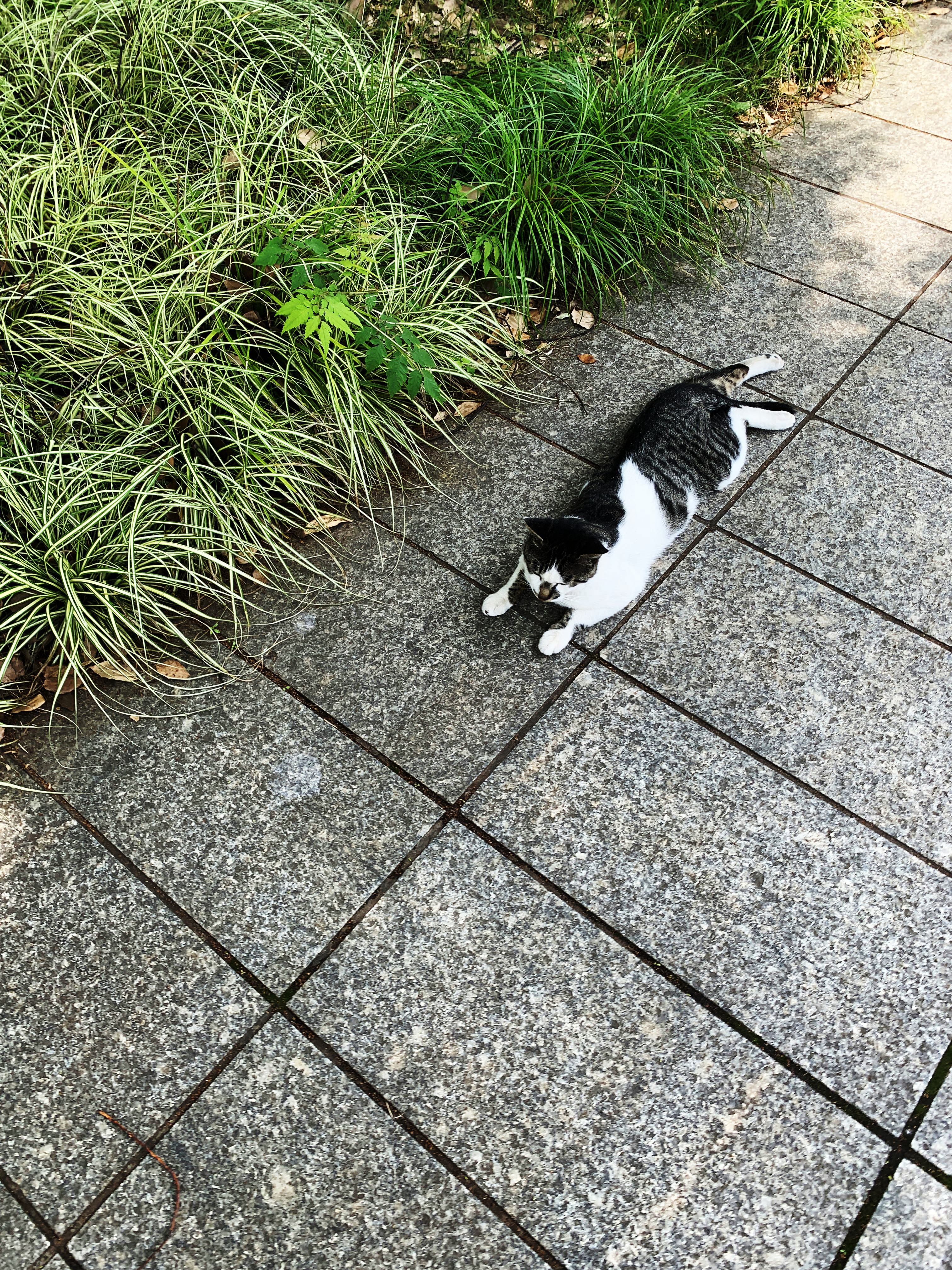
I extracted the quantization matrix from my cat.jpg,
and here’s what it looks like:
{
  0: [1, 1, 1, 2, 3, 4, 5, 6, 1, 1, 1, 2, 3, 4, 5, 6, 1, 1, 2, 3, 4, 5, 6, 7,
      2, 2, 3, 4, 5, 6, 7, 8, 3, 3, 4, 5, 6, 7, 8, 9, 4, 4, 5, 6, 7, 8, 9, 9,
      5, 5, 6, 7, 8, 9, 9, 9, 6, 6, 7, 8, 9, 9, 9, 9],
  1: [1, 1, 2, 4, 9, 9, 9, 9, 1, 2, 2, 6, 9, 9, 9, 9, 2, 2, 5, 9, 9, 9, 9, 9,
      4, 6, 9, 9, 9, 9, 9, 9, 9, 9, 9, 9, 9, 9, 9, 9, 9, 9, 9, 9, 9, 9, 9, 9,
      9, 9, 9, 9, 9, 9, 9, 9, 9, 9, 9, 9, 9, 9, 9, 9]
}
In JPEG, we usually deal with two separate quantization tables:
Luminance Table (Y) → This one is applied to the brightness part of the image, aka the Y channel in YCbCr. It’s where the human eye is most sensitive, so we compress it less aggressively.
Chrominance Table (Cb + Cr) → This one handles the color details. Our eyes aren’t super sensitive to color changes, so JPEG is more brutal here with compression. Hence, more aggressive quantization.
Technically, it’s possible to use more than three quantization matrices. But most real-world JPEGs stick to 2. Some encoders can assign a separate matrix to Cr too, so 3 total:
Table 0 → YTable 1 → CbTable 2 → Cr
But that’s rare and not supported by all decoders.
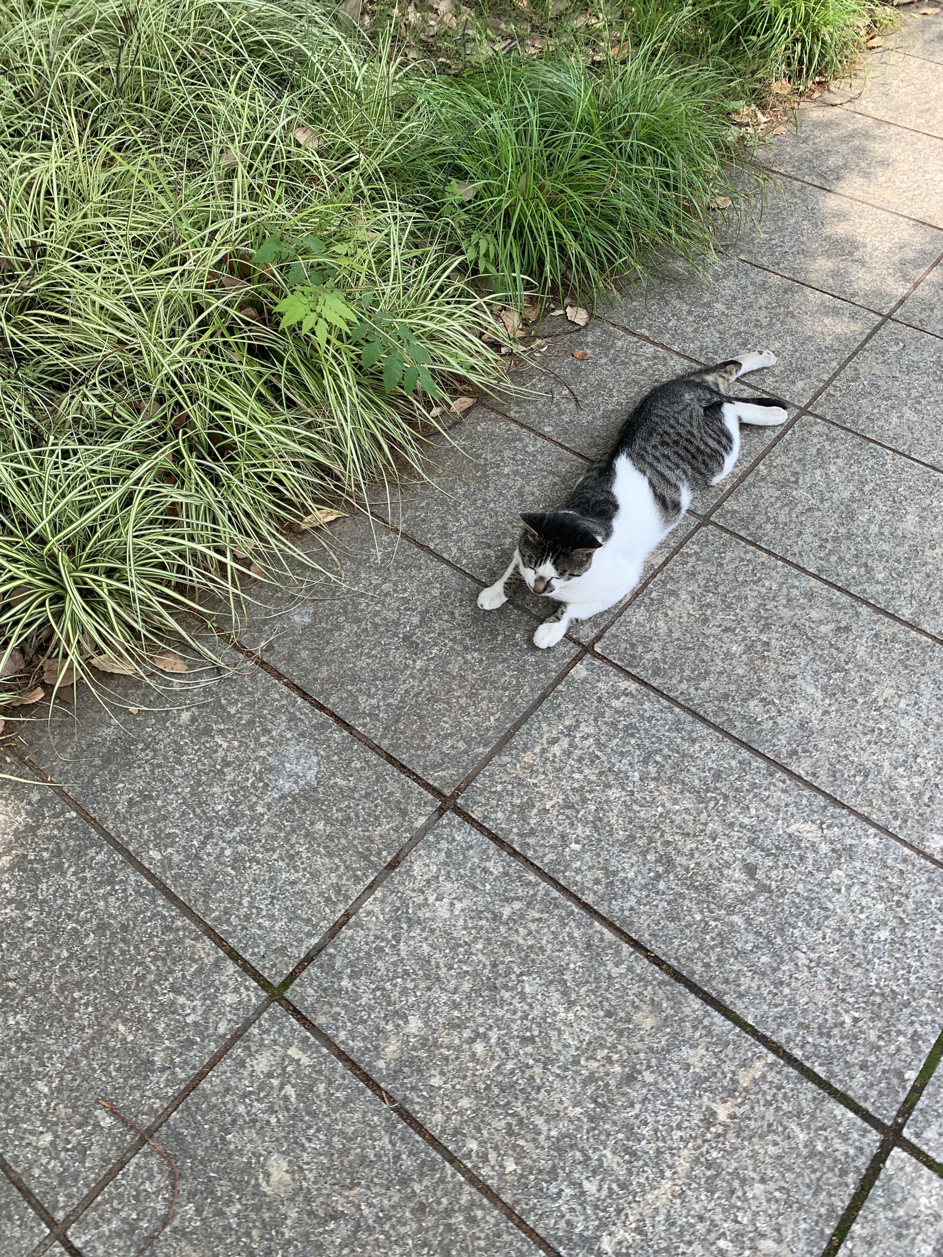
Visualize the quantization matrices:
Luminance Table (0):
- Starts with small values like
1,1,1,2, meaning little to no loss in low-frequency areas = sharp brightness details. - Higher-frequency entries gradually increase (e.g.,
8,9), so they compress more subtle details.
Chrominance Table (1):
- Starts slightly higher (
1,1,2,4), then quickly becomes saturated with9, meaning hardcore compression on color subtleties.
This JPEG encoder is smart. It compresses where the eye won’t notice (color), and protects where it will (brightness). This saves file size without making the lil kitten look like mashed pixels.
Click to preview the theme visualization
YCbCr
RGB is where each pixel has 3 values. But RGB ain’t perfect for compression. So JPEG goes with YCbCr.
1
2
3
Y  →  Luminance = Brightness
Cb →  Blue Chrominance = Blueness
Cr →  Red Chrominance = Redness
Since we notice brightness changes a lot, but don’t care much about slight shifts in color hue. So JPEG use a nice detailed matrix for Y, and a more aggressive, lossy one for Cb/Cr.
Each 8×8 block is three layers stacked:
1
2
3
Block 1: Y (brightness)
Block 2: Cb (blueness)
Block 3: Cr (redness)
Every 8×8 pixel “region” of your image gets split into three 2D 8×8 blocks: One for Y, one for Cb, one for Cr. If you think of the same 8×8 patch of your image, you have three separate 2D arrays (blocks):
                                ┌───────┐
                                │ Block │
                                │   Y   │  (brightness)
                                └───────┘
                                ┌───────┐
                                │ Block │
                                │  Cb   │  (blueness)
                                └───────┘
                                ┌───────┐
                                │ Block │
                                │  Cr   │  (redness)
                                └───────┘
They are like three 8x8 slices stacked on top of each other(like a small 8×8×3 cube). All three blocks occupy the same (x,y) area, just in different channels. JPEG applies quantization table 0 to Y and quantization table 1 to both Cb and Cr. So they compress differently.
If you zero out the Cb/Cr channels (just keep Y), you get a grayscale image - all structure, no color:
1
img.convert("YCbCr").split()[0].show()
Keeping only one channel at a time, here’s how cat.jpg appears in each:
Only blur one channel, and merge with others:
cat.jpg vs cat.png
JPEG used DCT, so it threw away some frequency data. JPEG’s lossy compression (especially DCT + quantization) makes it easier to embed hidden data in frequency space. JPEG is almost always 8-bit/channel, 0-255 shades of red, green, and blue, which make it lightweight, great for fast display or web use and good enough for human eyes.
PNG is better for exact pixel control, which is perfect for LSB watermarking or pixel-aligned visual hiding, but harder to stealth hide in frequency space, since it doesn’t use one. PNG can do 8 or 16 bits/channel, 0-65535 shades. This makes it super fine detail, but big size. Sharper gradients, better for editing, like medical or astronomical images.
For watermarking, higher bit-depth do give more room to hide stuff. And for 8-bit JPEG we have to be creative, like with DCT.
cat.jpg = 7.5 MB, while cat.png ≈ 34.7 MB (see size calculation for details).
Try converting cat.jpg to PNG and watch how it blows up in size. And convert it back to JPG:
1
2
3
convert cat.jpg cat_from_jpg.png
convert cat_from_jpg.png cat_rejpg.jpg
ls -lh cat.jpg cat_from_jpg.png cat_rejpg.jpg
Output (partial):
7.2M   cat.jpg
24M    cat_from_jpg.png
6.2M   cat_rejpg.jpg
cat_from_jpg.png: [24MB] for the PNG is still thicc! The cat’s pixels are living large and uncompressed. Big, lossless, preserves all bits as-is, including all JPG artifactscat_rejpg.jpg: [6.2MB] The file size shrinks back down. The image loses even more detail, especially in smooth areas or in the LSBs.
If you do this conversion repeatedly (JPG → PNG → JPG → PNG), the image quality keeps degrading, and the LSB stego data dies fast. What if cat.jpg gone wild - let’s try JPG → PNG → JPG → PNG, over and over again…
Here I tested for 100 times, just for fun:
1
2
3
4
5
6
7
8
9
10
11
12
13
14
15
16
17
18
19
Step 0: PNG size = 23649.4 KB
Step 1: JPG size = 4178.3 KB
Step 2: PNG size = 23332.9 KB
Step 3: JPG size = 4178.2 KB
Step 4: PNG size = 23335.3 KB
...
Step 29: JPG size = 4177.8 KB
Step 30: PNG size = 23339.2 KB
Step 31: JPG size = 4177.8 KB
Step 32: PNG size = 23339.2 KB
...
Step 109: JPG size = 4177.8 KB
Step 110: PNG size = 23339.2 KB
...
Step 167: JPG size = 4177.8 KB
Step 168: PNG size = 23339.2 KB
...
Step 199: JPG size = 4177.8 KB
Step 200: PNG size = 23339.2 KB
The first PNG is huge (23.6 MB), straight from the original JPG. First time it encoded as JPG: size drops to 4.1 MB - because JPEG throws out a lot of “irrelevant” detail.
When ping-pong between JPG and PNG:
JPG compresses hard, tossing subtle pixel values. After the first few rounds, all the “fine details” are already lost. Then JPEG can’t compress what isn’t there.
PNG tries to preserve the exact data it gets from that JPG, but, after just a few rounds, all further loss is minimal because the image is already “as compressed as JPEG wants.”
So we’d see:
PNG size = 23339.2 KB
JPG size = 4177.8 KB
again and again.
So here’s the final report:
JPG size = 7.4 MB -> 4.1 MB
After 100 rounds of recompression and re-encoding, the file stabilizes at ~4.1 MB and doesn’t shrink further. Also you can set quality=10 (instead of 85) to see much more dramatic continued loss/artifacts and a lower JPG size.
Applying DCT & Quantization on Y Channel Blocks
We’ll manually apply DCT to the Y channel, quantize it using a single matrix, and then visualize the DCT blocks - to explore what frequency components are present across the image.
(See freq_heatmap.py. Tinkering with pixel_shifting.py and subplot_mx.py would help better understand this script.)
Here we generate a grid of 64 heatmaps, each representing a single 8×8 DCT frequency block.
- Hot colors = strong frequencies (edges, details).
- Blue/red in corners = high frequency activity.
- Bright centers = strong low-freq (overall brightness).
Let’s recap and draw more ACSIIs:
Each image channel (Y, Cb, Cr) is split into many
8×8blocks.If your image is
512×512, then:512 / 8 = 64blocks per row- So in total:
64 × 64 = 4096 blocks per channel
 [Image chopped into 8 × 8 spatial blocks]

 ┌─────────────────────────── 512 px ────────────────────────────┐
 │  ░░░░  ░░░░  ░░░░  ░░░░  ░░░░  ░░░░  ░░░░  ░░░░  …  (64 blocks)│ ← Y channel
 │  ░░░░  ░░░░  ░░░░  ░░░░  ░░░░  ░░░░  ░░░░  ░░░░               │
 │  ░░░░  ░░░░  ░░░░  ░░░░  ░░░░  ░░░░  ░░░░  ░░░░               │
 │  … (64 rows of blocks) …                                      │
 └───────────────────────────────────────────────────────────────┘
         ↑
         512 px

 # 64 × 64 = 4096 blocks per channel (same grid for Cb and Cr).
Each
8×8block is transformed by DCT ➝ becomes 64 frequency coefficients (numbers).- One number = one type of frequency
- Top-left: low-freq (DC)
- Bottom-right: high-freq (super fine detail)
 [Zoom into *one* 8 × 8 block]

 Spatial pixel block (8×8)          DCT frequency plane (8×8)
 ┌───────────────┐                  ┌───────────────┐
 │ 123 130 132 … │  DCT →           │ DC  h1  h2 …  │  ← low-freq (DC) top-left
 │ 125 129 134   │                  │ v1  d1  d2 …  │
 │  …            │                  │ …        hi   │  ← hi-freq bottom-right
 └───────────────┘                  └───────────────┘
64 numbers = Coefficients describing how much of each sine-wave pattern is present.
Then it applies Quantization using a Quantization Matrix (Q):
1
quantized = np.round(dct_block / Q)
Large Q values ➝ more coefficients round to 0 ➝ information thrown away ➝ better compression.
Where the “64 little heat-map squares” come from
1
2
3
 fig, axs = plt.subplots(8, 8)
 ...
 ax.matshow(blocks[idx], cmap="seismic")
This told Matplotlib to show the first 64 spatial blocks (top-left 512 × 512 image area) after DCT + quantization:
Whole image First 8×8 grid of blocks visualized ┌─ ─ ─ ─ ─ ─ ─ ─┐ ┌───────────────┐ │ B0 B1 B2 … B7 │ → │ [B0][B1]…[B7] │ ‹── each cell is an 8 × 8 │ B8 B9 … B15 │ │ [B8][B9]… │ heat-map of coefficients │ … │ │ … │ └───────────────┘ └───────────────┘- Each coloured square is one 8×8 frequency matrix (quantized coefficients).
- We displayed the first 64 of them in an 8×8 collage.
We can also try different quantization matrices, to see how JPEG quantization matrix affects the frequency details of image blocks:
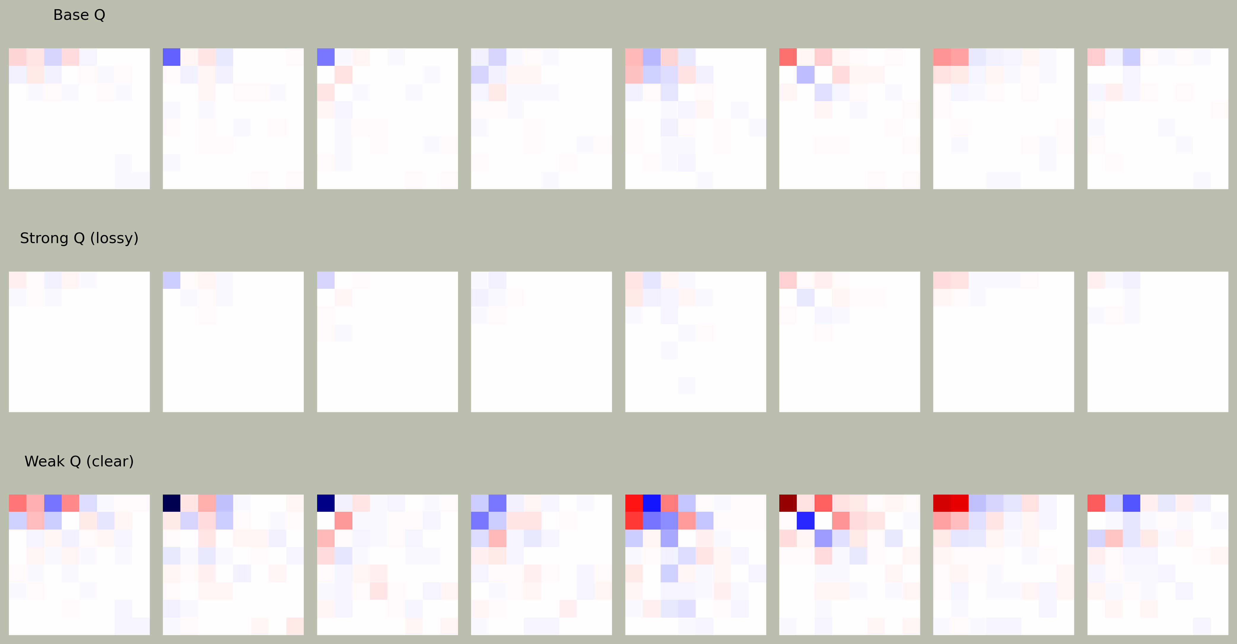
- Top Row: Base Q (×16) - moderate compression, keeping a healthy balance of detail and size.
- Middle Row: Strong Q (×50) - high compression, wiping out most of the fine detail (notice more red/blue blobs = fewer variations).
- Bottom Row: Weak Q (×5) - very fine detail preserved, sharper image but larger file.
So we’ve taken one channel (Y), applied DCT block-wise, quantized it using one matrix, and visualized what that does to the image.
Later we would:
- Embed info into these frequency spots (especially low-medium frequencies)
- Un-quantize and inverse DCT to rebuild a “watermarked” image
JSteg - DCT Embedding
Here we want to embedd 1 bit of our message (“uid:123456789”) into 1 block. This is very similar with LSB steganography process, but in DCT frequency space. Using DCT-space embedding keeps visual quality higher than doing LSB manipulation directly in the pixel values. We’re slicing that UID (converted into binary) into individual bits:
"uid:123456789" → '01110101 01101001 01100100...' (binary of ASCII)
And each 8×8 block’s [4][3] coefficient gets one bit of that:
- Block 0: embeds first bit
- Block 1: second bit … until the whole message is embedded.
To embed 80 bits, we need 80 DCT blocks.
For a 512 × 512 image, 262,144 pixels total, 512 × 512 image → (512 / 8)² = 64 × 64 = 4096 blocks total, so 4096 hidden bits possible if embed 1 bit per block.
For a 512 × 512 image, that’s 262,144 pixels total. Since each 8 × 8 block covers 64 pixels, we get (512 / 8)² = 64 × 64 = 4096 blocks total. So if we embed 1 bit per block, we can hide up to 4096 bits.
To calculate how many bytes:
- 1 pixel (grayscale) = 1 byte = 8 bits
- 1 pixel (RGB) = 3 bytes = 24 bits
But with JPEG, it’s not a 1:1 mapping - the DCT and quantization steps make it lossy. So if we embed 1 bit per 8×8 block in a 512×512 image,
that gives us 4096 bits = 512 bytes total. Not a ton of space, but enough for a UID, timestamp, maybe even a tag or signature.
Each DCT coefficient is stored as an integer, typically 8-12 bits internally (depends on compression level & quantization). We’re modifying only the LSB - 1 bit - of that coefficient. The cost in size is microscopic, just slightly tweaking the value already there. This won’t have the JPEG file get bigger, maybe a few bytes, but usually not noticeable. Especially if the compression is strong, and quantization masks the tiny changes. If we change many coefficients from small 0s to non-zero values, or introducing more “complexity” in the image = less compression efficiency, then that might make it larger. But we’re only flipping LSBs, which hardly affects the DCT’s magnitude spectrum.
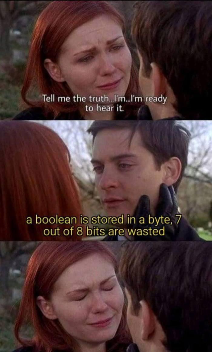
Redundancy
bool is a kind of redundancy. A bool only needs 1 bit:
0→ False1→ True
But in most languages (like Python, C, etc), a bool is stored in 1 byte = 8 bits. So when we use True in Python:
1
x = True
Behind the scenes, it’s:
00000001
The other 7 bits are wasted. That’s what we call storage redundancy or space overhead.
You know you wanna click it. It's a meme.
In LSB stego, we hate waste. we wanna use every juicy bit to hide our secrets. Here, redundancy is storing extra copies of the same data in case something is lost. Embedding same UID multiple times, or in multiple coefficient positions like [3][2], [5][5], [6][1], or across multiple channels (Y, Cb, Cr). Then even if one gets compressed or damaged (e.g., JPEG lossy), we still have backup.
Robustness
For DCT-based steganography, if we:
1
convert cat_dct_y.jpg -equalize cat_dct_y_eq.jpg
you probably won’t see any snow patterns like what we’ve did before in LSB embedding (LSB-in-pixels, which cause snow-like noise). Equalize is pixel-domain contrast stretch. It works by stretching histograms of pixel intensity values and highlighting visual differences in RGB pixels. But DCT stego happens in compressed DCT coefficients before the final pixel values even exist. Hidden changes are subtle, often invisible, unless done aggressively, like embedding too much (1+ bits per AC coefficient per block), or using high-frequency spots carelessly (e.g. [7][7]). Or the quantization matrix is too light (less compression).
This method is robustly invisible especially if embed one bit per block and stick to mid-range AC positions (like [4][3]), meanwhile keeping the image resaved in moderate JPEG quality (≥75).
Weak & attacks
This method (LSB embedding in the Y channel in DCT domain) is still very weak. There are plenty of attacks that can easily break or destroy the hidden data.
Lossy Compression (JPEG again)
If the image is recompressed at lower quality (say 90 → 50), it’ll:
- Re-quantize
- Kill subtle LSB tweaks
- Result: your secret bits gone
Image Filtering / Noise / Blur
- Gaussian blur or resize can smooth the DCT values
- Could change
[4][3]enough to flip the bit
Reformatting
- Changing from
.jpg→.png→.jpg= re-encode - Your frequencies: crushed
- Changing from
Histogram Equalization
- It redistributes brightness, could disturb Y channel values
Statistical Attacks
Like StegExpose can scan thousands of JPEGs looking for:
- Suspicious bias in LSBs
- Unnatural DCT patterns
- Low entropy where randomness is expected
Especially if you embed too much, it becomes detectable. That’s the paradox - the more you hide, the more you risk being exposed. Both stealth and strength get betrayed.
DCT Decoding
Now we’ve embedd “uid:123456789” in the Y channel. Do some attacks before decoding:
1
2
3
4
5
6
7
8
9
10
11
12
13
14
15
16
17
# Equalized
convert cat_dct_y.jpg -equalize cat_dct_y_eq.jpg
# JPEG Compression 40
convert cat_stego.jpg -quality 40 compressed.jpg
# JPEG Compression 35
convert cat_stego.jpg -quality 35 compressed.jpg
# JPEG Compression 30
convert cat_stego.jpg -quality 30 compressed.jpg
# JPEG Compression 20
convert cat_stego.jpg -quality 20 compressed.jpg
# Cropped (chop off first 128 pixels of height)
convert cat_stego.jpg -crop +0+128 cropped.jpg
# Blurred
convert cat_stego.jpg -blur 0x2 blurred.jpg
# Resized
convert cat_stego.jpg -resize 50% resized.jpg
Then decode the result by uncommenting mass decoding section in the script. Here’s the output (brief version):
1
2
3
4
5
6
7
8
9
10
11
12
13
14
15
16
17
18
[cat_stego.jpg]:
decoded_text = uid:123456789
[cat_dct_y_eq.jpg]:
decoded_text = hd:234$789
[blurred.jpg]:
decoded_text =
[compressed40.jpg]:
decoded_text = uid:123456789
[compressed35.jpg]:
decoded_text = uid:123456789
[compressed30.jpg]:
decoded_text =
[compressed20.jpg]:
decoded_text =
[cropped.jpg]:
decoded_text =
[resized.jpg]:
decoded_text =B@@!`@à
cat_stego.jpg- the intact original.We decode the full message here, exactly as expected.
Equalized - failed (weird string like
hd:234$789)Somewhat readable, but scrambled. Equalize isn’t meant to break JPEG-level DCT, but it adjusts pixel brightness nonlinearly, which can result in different DCT transforms and shifting LSBs. It doesn’t destroy the watermark with fire, but introduces bit noise.
Blurred - failed (blank)
Blurring smooths out local contrast and edges, which directly modifies the DCT coefficients, especially mid-frequency ones like
[4][3]. This “averaging” kills the details we were hiding bits in.JPEG Compression (survived until quality 35)
JPEG compression still preserves low-frequency DCT coefficients, especially in AC[4][3] where we’re embedding. Even with quantization rounding errors, the LSB of those lower-frequency coefficients is often preserved well under moderate compression. Quality 35 is roughly where the rounding starts really messing up our LSBs.
Cropped - failed (blank)
When embed bits, each bit is hidden in the LSB of the quantized DCT coefficient
quant[4][3]in each 8×8 block, in order (top left, row by row). Example: the first embedded bit is in the top-left block (at[0:8, 0:8]), the second is in the next block to the right ([0:8, 8:16]), and so on. When cropped off the top 128 pixels (rows) from the image, that means we’ve deleted the entire first 16 rows of blocks (128px / 8 = 16 blocks tall), including every block that held the first N bits.
So when the decoding code expects to start at the very first block of the original stego image, since those blocks are now GONE, the decoding script starts at a new (later) block - so it sees new data, or maybe all zeros, or even can’t recover anything that matches the original message structure.Resized - failed (garbage)
Resizing triggers image interpolation (e.g. bilinear or bicubic), which blends pixels between blocks, destroying the DCT block structure. As a result, the decoder still finds
[4][3]from each new block, but it’s garbage bits, henceB@@!.
TL;DR
Embedded in the single channel:
Y:
| Test | Status | Reason |
|---|---|---|
| Equalize | ✗ Noise | Nonlinear pixel shifts altered LSBs |
| Blur | ✗ Blank | High-freq lost, DCT flattened |
| JPEG q40-35 | ✓ Success | Low/mid-freq DCT survived |
| JPEG q30↓ | ✗ Blank | LSB got mangled |
| Crop | ✗ Blank | Bits in cropped blocks = gone |
| Resize | ✗ Garbage | New blocks, interpolated trash |
Cb (blue chroma):
- ✓
cat_stego_cb.jpg: Intact one, decoded. - ✗ All attacks like
blurred,compressed20,cropped,resized, and evencompressed35totally zero’d it. equalizeddid something funky: “`d:12345678”. So it altered the early bits a little (maybe due to contrast stretching of color).
Chroma channel watermarking is fragile under most processing. Equalization even slightly perturbs it, and JPEG recompression nukes it immediately.
Cr (red chroma):
- ✓
cat_stego_cr.jpg: Intact one, decoded. - ✗ Like before, every attack kills the payload.
equalizedagain gets weird:hd:04$39.
Cr behaves like Cb, very stealthy, doesn’t affect image visibly, but gets messed up easily by any processing that touches colors.
DCT multi-channel Enbedding & Decoding
Redundant Embedding Across Channels (Y, Cb, Cr)
Embed the exact same UID into Y, Cb, and Cr channel. All using the same coefficient position, like
[4][3]. Hiding three backup copies, so if one vault gets blown up (say Cb gets EQ’d), you can still recover from Y or Cr.Then on decode, check all three, and pick the one that gives a readable output. Or, do a majority vote per bit to reduce noise.
Redundant Embedding Within One Channel (Spread Across Positions)
Instead of embedding all bits in
[4][3]across blocks, spread them like:- 1st bit →
[3][2] - 2nd bit →
[5][3] - 3rd bit →
[2][1] - … and so on.
It can help hide better from certain attacks that target specific frequencies or locations.
- 1st bit →
Combine these two ideas would get you a layered, resilient watermark. Redundancy across channels and positions. Optionally add ECC to fix minor damage.
Majority vs Or
Actually the quick “majority” demo felt worse:
It reads the same bit from Y and Cb and Cr, then does
bit = 1 if sum≥2 else 0.If Y = 1, Cb = 0, Cr = 0 → majority ⇒ 0 ⇒ lose the bit.
So if chroma copies are “all-zero”, they actually out-vote the good Y copy.
Bit-wise OR (any channel can rescue):
bit = Y ∨ Cb ∨ Cr (i.e., 1 if any copy is 1). If a channel is destroyed to zeros, it can’t “over-rule” the good copy.
The output of this version is like:
1
2
3
4
5
6
7
8
9
10
11
12
13
14
15
[cat_dct.jpg]:
Y  : 0111010101101001011001000011101000110001001100100011001100110100
Cb : 0111010101101001011001000011101000110001001100100011001100110100
Cr : 0111010101101001011001000011101000110001001100100011001100110100
OR : 0111010101101001011001000011101000110001001100100011001100110100
ASCII-preview (OR): uid:123456789
uid:123456789

[compressed40.jpg]:
Y  : 0111010101101001011001000011101000110001001100100011001100110100
Cb : 0000000000000000000000000000000000000000000000000000000000000000
Cr : 0000000000000000000000000000000000000000000000000000000000000000
OR : 0111010101101001011001000011101000110001001100100011001100110100
ASCII-preview (OR): uid:123456789
uid:123456789
Yhas the real bits.Cb&Crmostly zeros (destroyed).ORkeeps the Y bits because1 OR 0 OR 0 = 1.- The preview shows the UID again.
It’s simple, more robust than majority when chroma tends to zero-out. But if noise flips a 0→1 in any channel you’ll get a false 1. Too fix this, add a tiny parity/ECC to catch rare flips.
Parity
| Term | TL;DR |
|---|---|
| Parity bit | A single extra bit you tack onto a chunk of data that tells you whether that chunk currently holds an even or odd number of 1-bits. |
| Even parity | You set the parity bit so the total 1-count becomes even. |
| Odd parity | You set it so the total 1-count is odd. |
| Job | Detect (not correct) any 1-bit error inside that chunk. If one bit flips, the parity no longer matches → “something went wrong”. |
It’s like a tiny “checksum” that only costs 1 bit per chunk.
Suppose each ASCII byte (8 bits) we embed is followed by one parity bit:
Encode phase
Count 1-bits in that byte → write an extra “even-ness” bit into the next block.
Decode phase
Re-count 1-bits you extracted. Compare with the parity bit. If mismatch, that byte got hit by at least one error. You can flag it or attempt a retry / ignore.
Parity detects, but can’t fix, a single-bit error. For correction we’d step up to Hamming(12, 8) or BCH(15, 11) - tiny ECCs that both detect and repair any 1-bit flub in each byte.
Let’s see how parity applies to "1234" example:
1
2
3
4
5
6
7
8
9
10
UID = '1234'

data_with_parity = []
for char in UID:
    # Convert char to ASCII integer
    byte = f"{ord(char):08b}"
    parity = byte.count("1") % 2      # even-parity
    data_with_parity.append(byte + str(parity))
bits = "".join(data_with_parity)
print(bits)
Take Each Character
"1"= ASCII49=00110001"2"= ASCII50=00110010"3"= ASCII51=00110011"4"= ASCII52=00110100- =>
00110001 00110010 00110011 00110100
Count 1s in Each Byte, Add Parity Bit
Even parity:
- If the count of 1s is even, add a
0 - If odd, add a
1
So the total number of 1s in (byte + parity) is always even.
"1":00110001→ Count of 1s = 3 (odd)- Parity bit = 1 (to make total even)
- Full:
00110001**1**(now 4 ones)
"2":00110010→ Count of 1s = 3 (odd)- Parity bit = 1
- Full:
00110010**1**
"3":00110011→ Count of 1s = 4 (even)- Parity bit = 0
- Full:
00110011**0**
"4":00110100→ Count of 1s = 3 (odd)- Parity bit = 1
- Full:
00110100**1**
- If the count of 1s is even, add a
Join All Together
So the stego bitstream will be:
 00110001  00110010  00110011  00110100
         ↓         ↓         ↓         ↓
 001100011 001100101 001100110 001101001
That’s 9 bits per char, instead of 8. (The last digit of each 9 is the parity bit.)
Parity lets you check for errors: If you decode a byte+parity and the total 1s is odd, you know a bit was changed.
While decoding and Checking Parity:
- Take every 9 bits: first 8 bits = data, 9th = parity.
Count the 1s in all 9 bits.
- If the total is even, probably OK.
- If the total is odd, something’s wrong (one bit likely got corrupted).
Weak
Parity can ONLY detect odd errors
- 1 bit error: Detected (parity broken)
- 2 bit errors in same chunk: Not detected (parity matches, but both bits are wrong)
- 3 bits flipped: Detected (again, odd number)
- 4 bits…: Not detected, and so on…
Parity can only tell you if there was an odd number of bit flips in each 9-bit chunk. If two bits (or any even number) get corrupted, the parity check passes, but the data is bad. Parity is not robust for targeted/strong attacks or heavy distortion. A true watermark system would use more advanced codes, like Hamming or Reed-Solomon, for error correction, not just detection.
Hamming Code
A classic error-correcting code (ECC) that not only detects errors, but can also correct single-bit errors. It works by adding multiple “parity bits” to your data, not just one. Each parity bit checks a different pattern of data bits, so when something flips, you can figure out which bit is wrong and fix it. If one bit gets corrupted (even in a big chunk), Hamming tells you exactly which bit and you can flip it back. If two bits are wrong, it usually at least detects “something’s up” (but can’t always fix).
Convert “1234” to Bits:
00110001 00110010 00110011 00110100Hamming (7,4) Example
Hamming (7,4) encodes 4 bits of data into 7 bits, adding 3 parity bits for error correction.
Let’s take the first 4 bits
0 0 1 1(from “1”)Positions:
1 2 3 4 5 6 7 P P D P D D D- P = Parity bit
- D = Data bit
So, mapping:
- bits 3, 5, 6, 7 are your data bits
Suppose data:
- d1 = 0 (bit 3)
- d2 = 1 (bit 5)
- d3 = 1 (bit 6)
- d4 = 0 (bit 7) (using next bit, let’s just show process)
Let’s encode “0011” using Hamming (7,4):
a. Fill the bits:
 Positions: 1 2 3 4 5 6 7
            P P D P D D D
            ? ? 0 ? 0 1 1
Assign D:
- 3: 0
- 5: 0
- 6: 1
- 7: 1
b. Calculate parity:
- Positions: 1 2 3 4 5 6 7
- Binary: 1 10 11 100 101 110 111
- Every parity bit is placed at a power-of-two position: 1, 2, 4.
Parity bit at position 1 (
P1):- Covers all positions where the least significant bit is 1.
- Binary:
1(1),11(3),101(5),111(7) - So: P1 (bit 1) covers 1,3,5,7: 1⊕3⊕5⊕7 = P1⊕0⊕0⊕1
Parity bit at position 2 (
P2):- Covers all positions where the second bit from the right is 1.
- Binary:
10(2),11(3),110(6),111(7) - So: P2 (bit 2) covers 2,3,6,7: 2⊕3⊕6⊕7 = P2⊕0⊕1⊕1
Parity bit at position 4 (
P4):- Covers all positions where the third bit from the right is 1.
- Binary:
100(4),101(5),110(6),111(7) - So: P4 (bit 4) covers 4,5,6,7: 4⊕5⊕6⊕7 = P4⊕0⊕1⊕1
Calculate (XOR for parity):
- P1: 0⊕0⊕1 = 1, so P1 = 1
- P2: 0⊕1⊕1 = 0, so P2 = 0
- P4: 0⊕1⊕1 = 0, so P4 = 0
Now we fill:
 Positions: 1 2 3 4 5 6 7
            1 0 0 0 0 1 1
So the codeword is: 1000011
Embed these bits as your watermark
You can replace the bits we used before (
quant[4][3]LSBs) with these Hamming-encoded bits. If a single bit flips (e.g., due to compression or cropping), Hamming lets you detect and correct it. On decode, you calculate the parity bits and spot the “bad” bit by position.
Reed-Solomon Code
Super-powerful, used in CDs, QR codes, satellites, SSDs, deep-space comms, bank card’s chip… Even Blu-ray Discs wouldn’t exist without it. Instead of just bits, it splits your data into “blocks” (symbols) and uses fancy math (polynomials over finite fields) to create redundant info. It can correct several errors at once. Even if whole pieces of data are missing, it reconstructs them. That’s why a scratched CD still plays.
- Hamming: Good for single-bit errors (like if 1 bit gets flipped).
- Reed-Solomon: Good for bursts of errors-multiple bits, or even whole bytes, nuked at once (like if a whole part of an image gets corrupted).
Suppose:
- You want to encode a 3-digit secret:
7, 3, 9 - We use a simple RS(5,3) code (5 total, 3 data, 2 extra)
- It’s like: you send
7, 3, 9, ?, ? - The last 2 “?” are check symbols, calculated cleverly (polynomials, but let’s skip the deep math for now)
Now, say your message gets trashed and arrives as:
7, XX, 9, XX, 2(whereXX= destroyed, but 2 is a check symbol that survived)- The receiver can rebuild the missing data using the remaining good symbols and those check symbols.
Data:      [ 7 3 9 ]
Check:     [ ?? ?? ]
Sent:      [ 7 3  9 c1 c2 ]
Errors:    [ 7 XX 9 XX c2 ]
Recovery:  [ 7 3  9 c1 c2 ]
Modern Watermarking
Legacy LSB (tested)
Old school: Flip LSBs in pixel values or DCT coefficients. Easy to implement, easy to break with heavy edits.
DCT/Block-Based Stego (tested)
Slightly more robust: Hide data in DCT blocks, usually in mid-frequency coefficients (not just
[4][3]- can be scattered). Can survive mild compression, but fails under heavy attack.Visible “Snow” Patterns
Douban’s “anti-leech”/”copy protection” overlays a partially visible pattern (the snow/lego effect we see when equalizing). This isn’t pure LSB, it’s an actual visible pattern, generated algorithmically, often tied to your UID/timestamp. The pattern is rendered on top of the image before you see/download it. It’s baked in, no magic decoding can reveal the data, but it’s easily seen with image enhancement.
Invisible Frequency/Watermark Techniques
- DCT domain with secret key: Data hidden in more complex patterns, possibly using pseudo-random positions, error correction, or even cryptographic keys.
- Spread Spectrum: Data is “spread” across many coefficients or pixels, not in a single place, very robust.
- Deep Learning Watermarks (SOTA): Watermarks embedded using neural nets, almost impossible to visually detect or remove without destroying the image.
Metadata/XMP Watermarks
Sometimes UIDs/timestamps are hidden in metadata chunks, not pixels. Easy to remove if you know where to look.
To Actually Destroy Modern Watermarks
A. For LSB/DCT/Oldschool:
- Recompress with JPEG quality <30-40 (as we tested, kills most weak marks).
- Resize (even by 1px), crop, or blur lightly.
- Equalize or histogram shift can sometimes help, but mostly just reveals.
- Color space shift (convert to/from grayscale, or shuffle RGB channels).
- Remove metadata:
exiftool -all= -overwrite_original img.jpg
B. For Visible Snow Patterns:
- Crop the pattern if it’s at the border.
- Heavy blur or median filter over just the snow area.
- Repaint or inpaint with Photoshop, GIMP, or even AI image restoration.
- Mask + background fill: Replace snow area with neighbor pixels.
C. For Advanced (Spread/Frequency/Deep Learning):
- Multiple attacks in combination: Resize + blur + crop + compress.
- Downscale/Upcale (e.g. 100%→90%→100%).
- Image-to-image with local AI (Denoising, Stable Diffusion outpainting).
- Paint over “signature” areas (if you can spot them).
- But if it’s really robust (deep learning watermark), you may need to just take a another shot(with nother camera) of your screen, but still not 100% robust.
nuke
(See nuke.py)
a. Optional: Crop the top N pixels
img.crop((0, N, W, H))
If the watermark pattern is embedded in a top header bar, this simple crop removes it cleanly.
Visual impact: zero loss for the main post content.
b. Downscale → Upscale
img.resize(0.96·size, Resampling.LANCZOS) and then scale it back up
Breaks the 1-pixel alignment of grid-based watermarking patterns by resampling.
Visual impact: barely noticeable.
c. Apply a Tiny Blur
ImageFilter.GaussianBlur(radius=1.3)
Gently averages out ±2-level brightness bumps - like the “snow” effect often used in LSB watermarks.
Visual impact: imperceptible.
d. Add Random ±1 Noise
np.random.randint(-1, 2, shape)
Introduces slight randomness to each pixel, disrupting any remaining UID bits hiding in low bits.
Visual impact: invisible.
e. Jitter (core)
1
2
3
4
5
6
jit_x, jit_y = 0.37, 0.19
img = img.transform(
    img.size,
    Image.AFFINE,
    (1, 0, jit_x, 0, 1, jit_y),
    resample=Image.Resampling.BICUBIC)
Image.AFFINE is a 2D transform. The tuple (1, 0, jit_x, 0, 1, jit_y) encodes an affine matrix:
  | 1  0  jit_x |
  | 0  1  jit_y |
This moves every pixel by a tiny amount: +0.37 px in x, +0.19 px in y (i.e., a subtle jitter). The transform “nudges” the whole image by a fractional pixel, not a full-pixel shift. The resampling (BICUBIC) blends/interpolates, so every pixel becomes a weighted sum of its neighbors. (I REALLY recommend OpenCV with Python By Example (Prateek Joshi) for this part.)
LSB-based overlays (snow/watermark) are extremely fragile - they depend on exact pixel alignment. Fractional-pixel jitter is like “shaking” the pixels just enough so their LSBs get totally changed after resampling. It’s NOT a round shift (which would leave the pattern), but a smooth blend. Almost no snow pattern can survive this, because the bits get mixed up, and the watermark “breaks apart.” Histogram equalization after this will reveal no more pattern - just noise made dramatic by equalisation:
You can randomize jit_x/jit_y per image for even more chaos. This trick works on any watermark that depends on precise pixel grid alignment - including some QR, snow, or even invisible text patterns.
Visual impact: nearly invisible.
f. (Optional) global 3×3 median to smooth the noise (optional)
img = img.filter(ImageFilter.MedianFilter(3))
Light median on the entire image after the jitter (radius = 1).
Visual impact: Kills isolated pixels but keeps UI text crisp.
g. Re-encode to JPEG at Quality ≈ 40 (or convert PNG → JPG)
img.save(q=40)
The heavy JPEG quantization at this level flattens mid-to-high frequency DCT coefficients where watermarks often live.
Visual impact: mild size/quality loss.
h. Strip Metadata
Optional extra exiftool -all= or let Pillow drop it on save
Completely removes any embedded metadata like EXIF, XMP, or custom UID fields.
Actually when we use Pillow (img.save(..., format="JPEG", ...)) to save a new JPEG, it does NOT copy over any of the original EXIF or metadata by default. The only thing in the file will be the image pixels and the minimal info needed to display it. So all the _clean.jpg files are already stripped of metadata. So NO need to run exiftool -all= ... on the new files unless you are handling with other formats like TIFFs or HEICs.
Visual impact: none.
Install deps:
1
2
pip install pillow numpy
sudo apt install -y libimage-exiftool-perl   # if you you're handling other formats like TIFFs or HEICs
Optionally strip metadata after save:
1
exiftool -all= -overwrite_original img.jpg
Nautilus Right-Click Magic (GNOME)
If you are in Linux and using GNOME, I highly recomend this right click trick - one click to nuke hidden watermark.
Install xclip and aftermark first:
1
2
sudo apt install -y xclip
pip install aftermark
Create the script folder (if it doesn’t exist):
1
mkdir -p ~/.local/share/nautilus/scripts
Create the script:
1
2
mkdir -p ~/.local/share/nautilus/scripts
nano ~/.local/share/nautilus/scripts/nuke
Paste:
1
2
3
4
5
#!/usr/bin/env bash
for src in "$@"; do
  dir=$(dirname "$src")
  nuke "$src" "$dir"
done
Then:
1
chmod +x ~/.local/share/nautilus/scripts/nuke
Now right-click a directory or multiple files, nuke would work instantly.
Same for exiftool, just paste (make sure you have sudo apt install -y libimage-exiftool-perl‘d):
1
2
3
4
!/usr/bin/env bash
for src in "$@"; do
  exiftool -all= -overwrite_original "$src"
done
Commands Cheat Sheet
peek at original dimensions
1
  identify -format "%wx%h\n" demo.jpg  # -> 1280x1707
Extract three channels:
1
2
3
  convert demo.png -channel R -separate r.png
  convert demo.png -channel G -separate g.png
  convert demo.png -channel B -separate b.png
Or one line:
1
  for c in R G B; do convert demo.png -channel $c -separate ${c}.png; done
This gives you
r.png,g.png,b.png(lowercase).Apply
-auto-level -contrast-stretch 1%x1%to each channel1 2 3
convert r.png -auto-level -contrast-stretch 1%x1% r_stretch.png convert g.png -auto-level -contrast-stretch 1%x1% g_stretch.png convert b.png -auto-level -contrast-stretch 1%x1% b_stretch.png
Or:
1
  for c in r g b; do convert ${c}.png -auto-level -contrast-stretch 1%x1% ${c}_stretch.png; done
Apply
-equalizeto each channel1 2 3
convert r.png -equalize r_eq.png convert g.png -equalize g_eq.png convert b.png -equalize b_eq.png
Or:
1
  for c in r g b; do convert ${c}.png -equalize ${c}_eq.png; done
Show all six outputs as a grid for comparison
1
  montage r_stretch.png g_stretch.png b_stretch.png r_eq.png g_eq.png b_eq.png -tile 3x2 -geometry +2+2 compare_grid.png
This makes a grid image to see which method/which channel pops the watermark.
lists every EXIF/IPTC/XMP tag
1
  exiftool -a -G -s demo.png
hunts for plaintext UID/TID blobs
1
  strings -n 8 demo.png | less
zsteg
1
2
3
4
  zsteg -E b1,r,lsb demo.png | strings
  zsteg -E b1,g,lsb demo.png | strings
  zsteg -E b1,b,lsb demo.png | strings
  zsteg -a demo.png | grep '123456789'
strip metadata (exiftool)
1
2
3
  exiftool -all= -overwrite_original demo.png
  # or
  exiftool -quiet -overwrite_original -all= *_clean.jpg
Lossy resize + quality dial-down
1
  convert demo.png -quality 92 -strip -resize 96% -colorspace sRGB demo_loss.jpg
-stripnixes metadata.Difference check
1
  compare -metric AE demo.png demo_loss.jpg demo_diff.png
blur
1
  convert demo.png -blur 0x2 demo_blur.png
Increase the 2 for a stronger blur.
That’s all for now, peace ooooout!
